ConvNeXt
The "Roaring 20s" of visual recognition began with the introduction of Vision Transformers (ViTs), which quickly superseded ConvNets as the state-of-the-art image classification model. A vanilla ViT, on the other hand, faces difficulties when applied to general computer vision tasks such as object detection and semantic segmentation. It is the hierarchical Transformers (e.g., Swin Transformers) that reintroduced several ConvNet priors, making Transformers practically viable as a generic vision backbone and demonstrating remarkable performance on a wide variety of vision tasks. However, the effectiveness of such hybrid approaches is still largely credited to the intrinsic superiority of Transformers, rather than the inherent inductive biases of convolutions. In this work, we reexamine the design spaces and test the limits of what a pure ConvNet can achieve. We gradually "modernize" a standard ResNet toward the design of a vision Transformer, and discover several key components that contribute to the performance difference along the way. The outcome of this exploration is a family of pure ConvNet models dubbed ConvNeXt. Constructed entirely from standard ConvNet modules, ConvNeXts compete favorably with Transformers in terms of accuracy and scalability, achieving 87.8% ImageNet top-1 accuracy and outperforming Swin Transformers on COCO detection and ADE20K segmentation, while maintaining the simplicity and efficiency of standard ConvNets.
TL;DR
ConvNeXt는 표준 ResNet을 출발점으로 잡고, Swin Transformer의 설계 선택을 하나씩 ConvNet 어휘로 옮겨 붙여가며 만든 순수 ConvNet backbone이다. self-attention을 전혀 쓰지 않고도 ImageNet-1K classification, COCO detection, ADE20K segmentation에서 동급 Swin Transformer와 같거나 더 나은 성능을 보이며, ImageNet-22K pretraining 후 ConvNeXt-XL이 87.8% top-1을 기록한다. 본 논문은 새 모듈을 제안하지 않는다. ConvNet과 Transformer의 성능 차이가 self-attention의 본질적 우위보다 training recipe와 macro/micro 설계 선택의 누적에서 온다는 것을 보인 것이 주요 기여다. 다만 등장하는 설계 요소가 모두 기존에 알려진 것들이며 개선 과정이 greedy하게 한 방향으로만 탐색됐기는 하다.
Background
2020년 ViT가 등장한 뒤 image classification의 SOTA는 빠르게 Transformer 쪽으로 넘어갔다. 다만 vanilla ViT는 global self-attention이 입력 크기에 대해 quadratic이라 고해상도 입력을 다루는 detection이나 segmentation에 그대로 쓰기 어렵다. Swin Transformer는 local window attention과 multi-stage hierarchy를 도입해 이 문제를 풀었는데, 이는 사실 ConvNet이 오래전부터 갖고 있던 sliding window, locality, 계층적 feature map 같은 inductive bias를 Transformer 안으로 다시 끌어온 것이다.
Swin이 잘 동작하니 ConvNet 대신 Transformer를 쓰자는 결론은 자연스럽지만, 저자가 문제 삼는 것은 그 성능 차이를 multi-head self-attention의 본질적 우위로 돌리는 해석이며, 이 통념에는 confound가 섞여 있다. ViT/Swin 계열은 architecture만 바꾼 게 아니라 AdamW, 긴 training schedule, 강한 data augmentation, stochastic depth 같은 training recipe도 함께 들여왔기 때문이다. system-level 비교(Swin vs ResNet)에서는 architecture 효과와 training 효과가 분리되지 않는다. 본 논문은 이 confound를 통제하면서, 표준 ResNet을 Swin과 같은 training recipe 아래 두고 architecture만 점진적으로 바꿔갈 때 성능 차이가 어디서 오는지를 추적한다.
Method
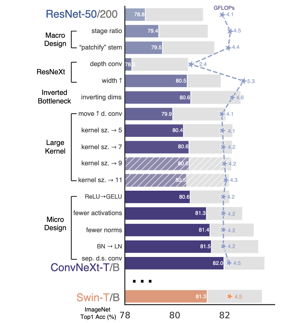 Modernization roadmap.
전체 구성은 ResNet-50을 Swin-T 쪽으로 단계적으로 옮기는 "modernization roadmap"이다. FLOPs를 대략 Swin-T 수준(약 )으로 유지하면서, 각 단계마다 하나의 설계 변경을 적용하고 ImageNet-1K top-1을 측정한다. ResNet-50 / Swin-T regime과 ResNet-200 / Swin-B regime 두 가지를 보는데, 본문은 전자를 기준으로 서술하고 후자는 결론이 일관됨을 appendix에서 확인한다. ResNet-50 regime의 각 수치는 random seed 3개 평균이다.
Training recipe 재구성
architecture를 건드리기 전에, ResNet-50을 ViT식 recipe로 다시 학습한다. 90 epoch에서 300 epoch으로 늘리고, AdamW, Mixup, CutMix, RandAugment, Random Erasing, Stochastic Depth, Label Smoothing을 적용한다. 이것만으로 ResNet-50이 76.1%에서 78.8%로 올라간다(+2.7%). 이 한 단계가 이후 architecture 변경들이 만들어내는 델타(대개 단계당 1% 미만)보다 크다는 점은 본 논문의 메시지에서 중요하다. ConvNet과 Transformer의 격차로 알려진 것의 상당 부분이 training 쪽에 있었다고 볼 수 있다.
Macro design
Swin-T의 stage 연산 비율 1:1:3:1을 따라, ResNet-50의 블록 수 (3, 4, 6, 3)을 (3, 3, 9, 3)으로 바꾼다. 78.8%에서 79.4%로 오른다. stem도 ResNet의 7×7 stride-2 conv + max pool 대신 ViT/Swin식 patchify, 즉 4×4 stride-4 non-overlapping conv로 교체한다(79.4% → 79.5%). stem을 더 단순한 patchify로 바꿔도 성능이 유지된다.
ResNeXt-ify & inverted bottleneck
3×3 conv를 depthwise conv로 바꾼다. depthwise conv는 채널별로 따로 동작해 spatial 방향만 섞는데, 저자는 이를 self-attention의 채널별 weighted sum과 유사한 spatial mixing으로 본다. depthwise conv와 1×1 conv의 조합은 spatial mixing과 channel mixing을 분리하며, 이는 Transformer block의 성질과 같다. depthwise conv 자체는 FLOPs와 정확도를 함께 떨어뜨리므로(78.3%), ResNeXt의 "use more groups, expand width" 원칙대로 채널 폭을 64에서 96(Swin-T와 동일)으로 늘려 80.5%로 회복한다.
이어서 inverted bottleneck을 적용한다. Transformer block의 MLP가 hidden dimension을 입력의 4배로 키우는 구조와, MobileNetV2 계열의 expansion ratio 4 inverted bottleneck이 같은 형태라는 관찰에서 출발한다. depthwise conv layer의 FLOPs는 늘지만 downsampling residual block의 1×1 shortcut conv에서 FLOPs가 크게 줄어 전체는 4.6G로 감소하고, 정확도는 80.5%에서 80.6%로 소폭 오른다. ResNet-200 regime에서는 이 단계의 이득이 더 커서(+0.79% vs +0.14%) regime에 따라 효과 크기가 달라진다.
Large kernel
large kernel을 쓰려면 먼저 depthwise conv layer를 블록 위쪽으로 올려야 한다. Transformer가 MSA를 MLP 앞에 두는 것과 같은 배치이며, inverted bottleneck에서는 무겁고 비효율적인 모듈(MSA, large-kernel conv)이 채널 수가 적은 위치에 오고 dense한 1×1 conv가 연산을 담당하게 하는 자연스러운 선택이다. 이 재배치는 FLOPs를 4.1G로 낮추면서 정확도를 79.9%로 일시 하락시킨다. 그 상태에서 kernel size를 3, 5, 7, 9, 11로 키워보면 7×7에서 80.6%로 회복하고 그 이상에서는 saturate한다. ResNet-200 regime에서도 7×7을 넘어 더 키울 때 추가 이득이 없다.
Micro design
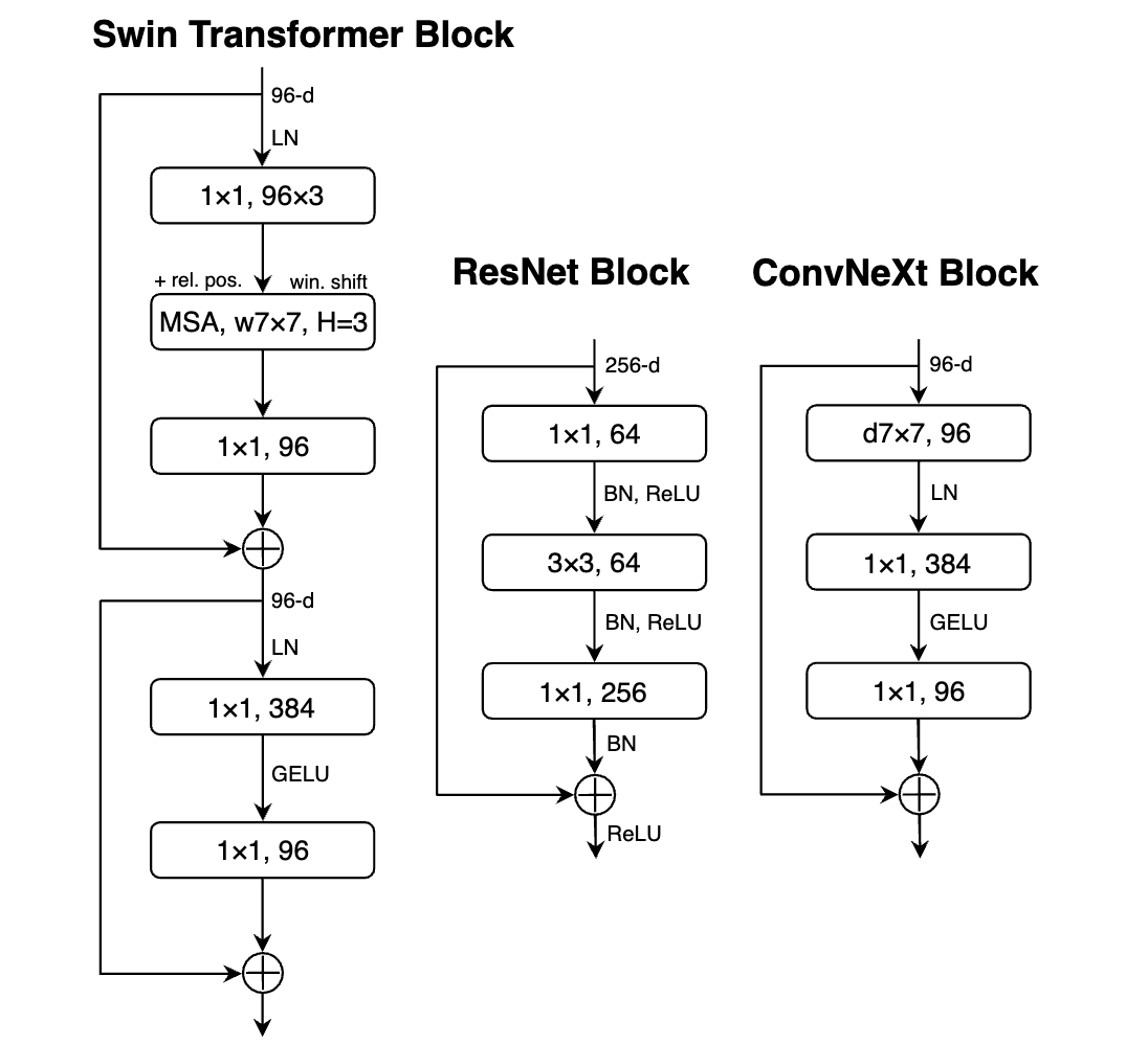 Block designs.
layer 수준의 변경들이 이어진다. ReLU를 GELU로 바꾸면 정확도는 80.6%로 그대로다. activation 수를 줄여 residual block 안에서 두 1×1 conv 사이의 GELU 하나만 남기면 81.3%로 0.7% 오르는데, ConvNet이 conv마다 activation을 붙이던 관행과 달리 Transformer block은 MLP 안에 activation이 하나뿐이라는 차이를 옮긴 것이다. normalization도 같은 방식으로 줄여 BN 하나만 남기면 81.4%가 되고, 이 시점에서 이미 Swin-T를 넘는다. BN을 LN으로 교체하면 81.5%로 소폭 더 오른다. 원래 ResNet에 LN을 그대로 넣으면 성능이 나빠진다고 알려져 있지만, 위 변경들을 모두 누적한 상태에서는 LN으로 학습에 문제가 없다.
마지막으로 downsampling을 분리한다. ResNet은 각 stage 시작 블록의 stride-2 conv로 downsampling을 처리하지만, Swin처럼 stage 사이에 별도의 2×2 stride-2 conv layer를 둔다. 이대로는 학습이 발산하는데, 해상도가 바뀌는 지점마다 LN을 추가하면 안정화된다(stem 뒤, 각 downsampling layer 앞, 마지막 global average pooling 뒤). 이 단계로 82.0%에 도달하며 Swin-T의 81.3%를 넘고, 이 구성이 ConvNeXt-T가 된다.
전체 modernization 과정의 단계별 수치를 보면 다음과 같다 (위의 Modernization roadmap과 동일).
| 단계 | IN-1K top-1 | GFLOPs |
|---|---|---|
| ResNet-50 (PyTorch) | 76.1 | 4.1 |
| + recipe 개섲 | 78.8 | 4.1 |
| + stage ratio | 79.4 | 4.5 |
| + patchify stem | 79.5 | 4.4 |
| + depthwise conv | 78.3 | 2.4 |
| + width 96 | 80.5 | 5.3 |
| + inverted bottleneck | 80.6 | 4.6 |
| + depthwise 위로 이동 | 79.9 | 4.1 |
| + 7×7 kernel | 80.6 | 4.2 |
| + GELU / fewer activations | 81.3 | 4.2 |
| + fewer norms | 81.4 | 4.2 |
| + BN→LN | 81.5 | 4.5 |
| + separate downsampling (ConvNeXt-T) | 82.0 | 4.5 |
| Swin-T (참고) | 81.3 | 4.5 |
블록 구조 자체도 단순해져서, depthwise 7×7 conv, LN, 1×1 conv(채널 4배 확장), GELU, 1×1 conv(축소)가 하나의 residual block을 이루며, shifted window attention이나 relative position bias 같은 특수 모듈이 없다. fully-convolutional이라 해상도를 바꿀 때 patch size를 조정하거나 position bias를 interpolate할 필요도 없다.
Results
ImageNet-1K에서 ConvNeXt-T/S/B/L은 동급 Swin을 전반적으로 앞선다고 보고한다. ConvNeXt-T가 82.1%로 Swin-T(81.3%)보다 0.8% 높고, ConvNeXt-B는 384² 입력에서 85.1%로 Swin-B(84.5%)를 0.6% 앞서면서 inference throughput은 12.5% 높다(95.7 vs 85.1 image/s). 특수 모듈이 없어 해상도가 올라갈수록 throughput 이점이 커진다.
| model | image size | #param | FLOPs | throughput | IN-1K top-1 |
|---|---|---|---|---|---|
| Swin-T | 224² | 28M | 4.5G | 757.9 | 81.3 |
| ConvNeXt-T | 224² | 29M | 4.5G | 774.7 | 82.1 |
| Swin-B | 384² | 88M | 47.1G | 85.1 | 84.5 |
| ConvNeXt-B | 384² | 89M | 45.0G | 95.7 | 85.1 |
| ConvNeXt-L | 384² | 198M | 101.0G | 50.4 | 85.5 |
ImageNet-22K pretraining 결과는 inductive bias 논쟁과 직접 맞물려 있다. ViT 계열이 inductive bias가 약해서 대규모 pretraining에서 ConvNet보다 유리하다는 통념이 있는데, 22K로 pretrain한 ConvNeXt는 동급 Swin과 같거나 더 나은 성능을 보이며 ConvNeXt-XL이 384²에서 87.8%에 도달한다. 충분히 현대화된 ConvNet이라면 대규모 데이터에서도 Transformer에 밀리지 않는다고 볼 수 있다. ImageNet-1K에서 advanced module(Squeeze-and-Excitation)과 progressive training을 쓰는 EfficientNetV2-L이 더 높지만, 22K pretraining을 붙이면 ConvNeXt가 그마저 앞선다고 한다.
downstream에서도 backbone으로서의 우위가 이어지는데, COCO에서 Mask R-CNN과 Cascade Mask R-CNN backbone으로 쓸 때 동급 Swin과 같거나 높은 box/mask AP를 보이고, 22K pretrained 대형 모델에서는 격차가 더 벌어져 ConvNeXt-B가 Swin-B 대비 +1.0 AP 수준까지 간다. ADE20K segmentation도 UperNet backbone으로 거의 모든 capacity에서 Swin을 앞선다.
효율 쪽 결과는 직관과 어긋나는데, depthwise conv를 많이 쓰는 모델은 같은 FLOPs에서 느리고 메모리를 더 쓴다고 알려져 있지만, ConvNeXt의 inference throughput은 Swin과 같거나 높고 학습 메모리는 더 적다(Cascade Mask R-CNN 기준 ConvNeXt-B 17.4GB vs Swin-B 18.5GB). A100에서 TF32와 channel-last memory layout을 쓰면 격차가 더 커져 Swin 대비 최대 약 49% 높은 throughput을 보인다고 한다. 이 효율 이점은 self-attention과 무관하게 local computation이라는 ConvNet inductive bias에서 온다는 것이 저자의 해석이다.
robustness 평가도 별도 모듈이나 추가 fine-tuning 없이 ImageNet-A/R/Sketch/C에서 경쟁력 있는 수치를 보인다. 22K data를 쓴 ConvNeXt-XL이 ImageNet-A/R/Sketch에서 각각 69.3/68.2/55.0%로 강한 domain generalization을 보고한다. isotropic 변형도 함께 실험하는데, downsampling 없이 14×14 해상도를 끝까지 유지하는 ViT식 구조에 ConvNeXt block을 넣어도 동급 ViT와 거의 같은 성능을 내, block 설계가 non-hierarchical 구조에서도 작동함을 확인한다.
Limitations
task 다양성이 주요 한계점인데, 평가가 classification과 dense prediction에 집중돼 있어 cross-attention으로 modality 간 상호작용을 모델링하는 multi-modal learning이나 discretized/sparse/structured output이 필요한 task에서는 Transformer가 더 유연할 수 있다고 언급한다. attention이 주는 유연성을 포기한 trade-off는 이 논문의 실험 범위에서는 측정되지 않는다.
또 각 단계의 델타가 작다. recipe 변경이 +2.7%인 데 비해 architecture 변경은 대개 단계당 1% 미만이고, ResNet-50 regime의 seed 표준편차가 0.1~0.2% 수준이라 일부 단계(patchify stem의 +0.1%, inverted bottleneck의 +0.1%)는 noise와 구분하기 어렵다. 최종 ConvNeXt-T가 Swin-T를 0.7% 앞서는 결론은 좋지만, 개별 설계 선택의 기여를 단독으로 신뢰하기는 어렵기 때문에 그냥 누적 효과로 읽는 편이 맞다.
등장하는 모든 설계 요소가 새롭지 않다는 점도 저자가 스스로 밝혔는데, depthwise conv, inverted bottleneck, large kernel, LN, patchify는 지난 10년간 개별적으로 연구돼 온 것들이고, 따라서 본 논문의 기여는 이를 한 ConvNet 안에 모아 controlled하게 검증한 데 있다고 볼 수 있다.
Thoughts
ViT 등장 이후 한동안 새 backbone의 우위가 architecture 덕인지 training 덕인지 구분되지 않은 채 보고됐는데, recipe를 고정하고 architecture만 바꾸는 것 만으로도 격차의 상당 부분이 사라진다는 결과를 통해 이후 backbone 논문을 읽을 때 system-level 수치를 그대로 받지 않게 만드는 기준점이 되었다고 생각한다.